- Derive the Born–Oppenheimer approximation in the form relevant for lattice dynamics and identify the small mass-ratio parameter behind it.
- Set up the displacement field for a crystal with a basis and expand the effective nuclear potential about equilibrium.
- Define coupling constants, state their symmetry and translational-invariance constraints, and write the harmonic equations of motion.
- Reduce the real-space equations of motion to a dynamical-matrix eigenvalue problem using a plane-wave ansatz.
- Count vibrational branches and classify acoustic, optical, longitudinal, and transverse modes.
5.1 Why Lattice Dynamics Matters for Thermal Physics
A rigid lattice is not enough to understand the thermal behavior of a solid. At finite temperature, atoms fluctuate about their equilibrium positions, and these collective motions are essential for specific heat, thermal expansion, sound propagation, and thermal conductivity, especially in insulators and semiconductors. The dynamical properties of the lattice also enter dielectric response, superconductivity, and inelastic light and neutron scattering. In this lecture we build the general harmonic formalism that makes these phenomena calculable.
5.2 Born–Oppenheimer Approximation and Effective Potential for the Nuclei
The first simplification is not yet specific to crystals. A solid is a coupled quantum system of electrons and nuclei, so in principle one should solve the full many-body Schrödinger equation for both at once. The reason this is usually not attempted directly in lattice dynamics is the large mass difference between electrons and nuclei: the electronic degrees of freedom adjust much faster than the nuclear ones. This scale separation motivates the Born–Oppenheimer, or adiabatic, approximation.
5.2.1 Full Electron–Nucleus Hamiltonian
We begin from the non-relativistic Coulomb Hamiltonian for \(N_e\) electrons and \(N_n\) nuclei:
with \[ \begin{aligned} T_e &= \sum_{i=1}^{N_e}\frac{\mathbf p_i^2}{2m_{\mathrm e}},\\ T_{\mathrm{ion}} &= \sum_{k=1}^{N_n}\frac{\mathbf P_k^2}{2M_k},\\ V_{ee} &= \sum_{i<j}\frac{e^2}{4\pi\varepsilon_0|\mathbf r_i-\mathbf r_j|},\\ V_{nn} &= \sum_{k<l}\frac{Z_k Z_l e^2}{4\pi\varepsilon_0|\mathbf R_k-\mathbf R_l|},\\ V_{en} &= -\sum_{i,k}\frac{Z_k e^2}{4\pi\varepsilon_0|\mathbf r_i-\mathbf R_k|}. \end{aligned} \]
Here \(T_e\) represents the kinetic energy of the electrons, \(T_{\mathrm{ion}}\) the kinetic energy of the nuclei, \(V_{ee}\) the interaction among the electrons, \(V_{nn}\) the interaction among the nuclei, and \(V_{en}\) the interaction among electrons and nuclei.
The exact stationary problem is therefore \[ H\Psi({\mathbf r_i},{\mathbf R_k})=E\Psi({\mathbf r_i},{\mathbf R_k}). \]
5.2.2 The Small Parameter
To see why the approximation is controlled, it is useful to measure lengths in Bohr radii and energies in Hartree units. In these atomic units the Hamiltonian can be written schematically as
The adiabatic Hamiltonian \(H_a\) contains the electronic kinetic energy and all Coulomb terms, but not the nuclear kinetic energy. The only small parameter that remains in the nuclear kinetic term is the mass ratio \(m_{\mathrm e}/M_k\), which ranges from about \(1/1836\) for hydrogen to much smaller values for heavier nuclei. Thus the nuclear kinetic energy is naturally treated as a slow perturbation of the electronic problem.
A simple classical estimate expresses the same idea. Forces exerted between electrons and nuclei are equal and opposite, so typical accelerations scale as \[ M_k\ddot{\mathbf R}_k \sim m_{\mathrm e}\ddot{\mathbf r}_i. \] The nuclei therefore move much more slowly than the electrons. In a harmonic restoring potential the characteristic nuclear frequencies scale as \[ \omega \propto \sqrt{\frac{m_{\mathrm e}}{M_k}}, \] when expressed in electronic atomic units.
5.2.3 Electronic Problem at Fixed Nuclei
Now freeze the nuclei at some instantaneous configuration \({\mathbf R_k}\) and group all remaining terms except \(T\) into the adiabatic Hamiltonian \[ H_a({\mathbf r_i};{\mathbf R_k}) = T_e+V_{ee}+V_{en}+V_{nn}. \]
For each fixed nuclear configuration one solves the electronic eigenvalue problem
The eigenvalues \(U_{\mathrm{el},s}({\mathbf R_k})\) are electronic energy surfaces as functions of the nuclear coordinates. In lattice dynamics, the most important one is usually the ground-state surface \(U_{\mathrm{el},0}({\mathbf R_k})\).
5.2.4 Expansion of the Full Wavefunction
The exact total wavefunction may be expanded in the electronic basis: \[ \Psi({\mathbf r_i},{\mathbf R_k}) = \sum_s \chi_s({\mathbf R_k}) \psi_s({\mathbf r_i};{\mathbf R_k}). \]
Substituting this into the full Schrödinger equation and projecting onto an electronic state yields a set of coupled nuclear equations. The only nontrivial point is that the nuclear kinetic-energy operator acts both on the nuclear amplitudes \(\chi_s\) and on the \({\mathbf R_k}\)-dependence of the electronic states \(\psi_s\). This produces derivative couplings between different electronic surfaces. Writing \[ \mathbf d_{ts}^{(k)} = \left\langle \psi_t \middle| \nabla_{\mathbf R_k}\psi_s \right\rangle_{\mathbf r}, \qquad \tau_{ts}^{(k)} = \left\langle \psi_t \middle| \nabla_{\mathbf R_k}^2\psi_s \right\rangle_{\mathbf r}, \] one obtains the exact coupled equations \[ \sum_s \left\{ -\sum_k \frac{\hbar^2}{2M_k} \left[ \delta_{ts}\nabla_{\mathbf R_k}^2 +2\mathbf d_{ts}^{(k)}\cdot\nabla_{\mathbf R_k} +\tau_{ts}^{(k)} \right] +\delta_{ts}U_{\mathrm{el},s}({\mathbf R_k}) \right\} \chi_s = E\chi_t. \]
5.2.5 Born–Oppenheimer Approximation
The Born–Oppenheimer approximation assumes that nuclear motion is slow enough that transitions between different electronic surfaces are negligible. Mathematically, one neglects the non-adiabatic couplings and keeps only one electronic surface, typically the ground state \(s=0\). Then the nuclear problem reduces to
This is the precise meaning of the statement that the nuclei move in an effective potential: the potential energy surface is the electronic ground-state energy as a function of all nuclear coordinates. The electronic subsystem is still essential; its ground-state energy determines the forces acting on the nuclei at each instantaneous nuclear configuration.
5.2.6 Transition to the Harmonic Approximation
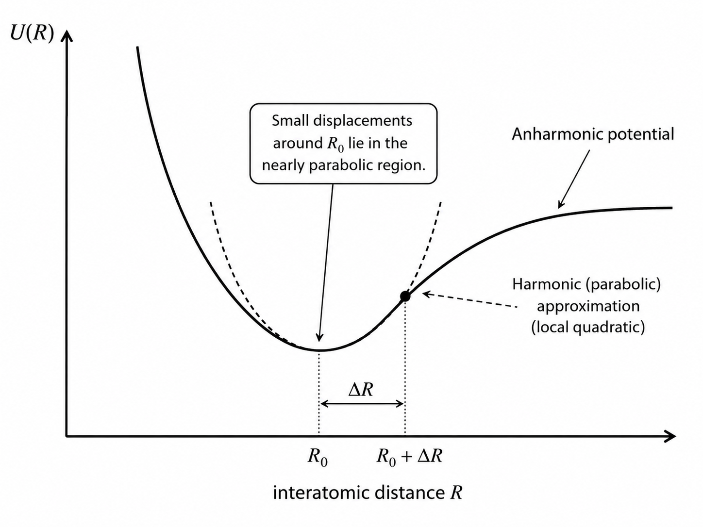
The Born–Oppenheimer approximation has now reduced the problem to nuclear motion on a multidimensional potential-energy surface. For lattice dynamics, the next step is to specialize to a periodic equilibrium crystal structure and assume that the nuclei perform only small oscillations about it. Then \(U_{\mathrm{el},0}({\mathbf R_k})\) can be expanded in powers of the nuclear displacements. Keeping only terms up to second order gives the harmonic approximation, which is the central working model of this lecture.
5.3 Geometry and Indexing of a Crystal with a Basis
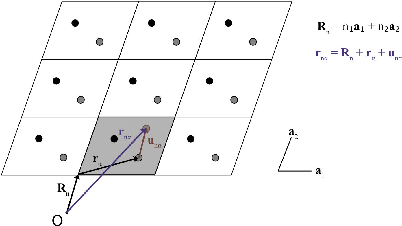
For a crystal with \(r'\) atoms in the primitive cell, we label cells by Bravais-lattice vectors \(\mathbf R_n\) and basis atoms by \(\alpha=1,\dots,r'\). The equilibrium position of atom \(\alpha\) in cell \(n\) is
and its instantaneous position is
The displacement field \(\mathbf u_{n\alpha}(t)\) is the central dynamical variable of the theory.
5.4 Harmonic Approximation and Coupling Constants
Within the Born–Oppenheimer approximation, the effective potential is the electronic ground-state energy evaluated at the instantaneous nuclear coordinates.
To describe lattice vibrations, we expand the total energy around the equilibrium atomic positions. For a function of a single variable, the Taylor expansion about an equilibrium point \(x_0\) is
\[ f(x)=f(x_0) +\left.\frac{df}{dx}\right|_{x_0}(x-x_0) +\frac12 \left.\frac{d^2f}{dx^2}\right|_{x_0}(x-x_0)^2+\cdots \]
At equilibrium, the first derivative vanishes:
\[ \left.\frac{df}{dx}\right|_{x_0}=0. \]
The leading correction is therefore quadratic, giving the familiar harmonic oscillator potential.
Now, in the context of the Born–Oppenheimer PES, the expansion yields
Here \(n,m\) label the Bravais lattice cells of the crystal, while \(\alpha,\beta\) label the atoms within the basis of each unit cell. The Cartesian indices \(i,j\in\{x,y,z\}\) specify the direction of the displacement. Thus \(u_{n\alpha i}\) denotes the displacement of atom \(\alpha\) in cell \(n\) along direction \(i\). The coefficients \(C^{m\beta j}_{n\alpha i}\) couple two such displacement coordinates and form the multidimensional generalization of the spring constant of a harmonic oscillator.
At equilibrium the linear term vanishes, because the first derivatives of the potential are zero there. Keeping only the quadratic term defines the harmonic approximation. The coefficients \(C^{m\beta j}_{n\alpha i}\) are the coupling constants: they have the dimensions of spring constants and generalize the single spring constant of a harmonic oscillator to a many-degree-of-freedom crystal.
5.4.1 Symmetry and Translational Invariance
Because mixed partial derivatives commute, \[ C^{m\beta j}_{n\alpha i} = C^{n\alpha i}_{m\beta j}. \]
Because a rigid translation of the entire crystal cannot generate restoring forces, the coupling constants satisfy the sum rule \[ \sum_{m,\beta} C^{m\beta j}_{n\alpha i}=0. \]
Finally, in an ordered crystal translational symmetry implies \[ C^{m\beta j}_{n\alpha i} = C^{(m-n)\beta j}_{0\alpha i}, \] so the couplings depend only on the difference between cell labels, not on absolute position.
A particularly useful equivalent form of the harmonic potential is \[ U_{\mathrm{el}}^{\mathrm{harm}} = \frac14 \sum_{n,\alpha}\sum_{m,\beta} \left[ (\mathbf u_{n\alpha}-\mathbf u_{m\beta})\cdot\nabla \right]^2 \phi(\mathbf r^0_{n\alpha}-\mathbf r^0_{m\beta}). \]
5.4.2 Pair-Potential Interpretation
Within the Born–Oppenheimer approximation, the electrons adjust instantaneously to the nuclear positions, so the nuclei move on an electronic potential energy surface (PES) \(U_{\mathrm{el}}(\{\mathbf r_{n\alpha}\})\), which depends on all atomic coordinates. In general this is a complicated many-body function. A common and physically intuitive approximation is to assume that the total energy can be written as a sum of effective pair interactions between atoms:
\[ U_{\mathrm{el}} = \frac12 \sum_{n,\alpha}\sum_{m,\beta} \phi(\mathbf r_{n\alpha}-\mathbf r_{m\beta}). \]
Here, \(\phi(\mathbf r_{n\alpha}-\mathbf r_{m\beta})\) is the effective interaction potential between atoms \((n,\alpha)\) and \((m,\beta)\), depending only on their separation vector. The factor \(1/2\) avoids double counting atomic pairs.
To study lattice vibrations, the atomic positions are written as small displacements about equilibrium:
\[ \mathbf r_{n\alpha} = \mathbf r^0_{n\alpha} + \mathbf u_{n\alpha}. \]
The separation vector between two atoms becomes
\[ \mathbf r_{n\alpha}-\mathbf r_{m\beta} = (\mathbf r^0_{n\alpha}-\mathbf r^0_{m\beta}) + (\mathbf u_{n\alpha}-\mathbf u_{m\beta}). \]
Expanding the pair potential in a Taylor series with respect to the relative displacement \(\delta\mathbf r=\mathbf u_{n\alpha}-\mathbf u_{m\beta}\) gives
\[ \phi(\mathbf R+\delta\mathbf r) \simeq \phi(\mathbf R) + (\delta\mathbf r\cdot\nabla)\phi(\mathbf R) + \frac12 \left[ (\delta\mathbf r\cdot\nabla) \right]^2 \phi(\mathbf R), \]
where
\[ \mathbf R = \mathbf r^0_{n\alpha}-\mathbf r^0_{m\beta}. \]
At equilibrium the linear term vanishes, and retaining only quadratic terms yields the harmonic approximation in the form
\[ U_{\mathrm{el}}^{\mathrm{harm}} = \frac14 \sum_{n,\alpha}\sum_{m,\beta} \left[ (\mathbf u_{n\alpha}-\mathbf u_{m\beta})\cdot\nabla \right]^2 \phi(\mathbf r^0_{n\alpha}-\mathbf r^0_{m\beta}). \]
This expression makes it explicit that the harmonic energy depends only on relative displacements between atoms, consistent with translational invariance of the crystal.
5.4.3 Interpretation
This form makes the physics transparent: only relative displacements matter. A rigid translation leaves all displacement differences unchanged and therefore costs no energy.
5.4.4 Range of Validity
The harmonic approximation is controlled by the size of the displacement relative to the lattice spacing. It is excellent for sufficiently small oscillations near equilibrium. At elevated temperatures, however, atomic displacements can become a non-negligible fraction of the lattice constant, and deviations from a purely quadratic potential become important. Such deviations are called anharmonic effects and will be needed later for thermal expansion and finite thermal conductivity.
5.4.5 Brief Remark on Microscopic Meaning
For central pair forces, the restoring force depends strongly on the component of the relative displacement along the line joining the atoms. This is why bond geometry enters lattice dynamics so directly, even within a harmonic description.
5.5 Equations of Motion in Real Space
The kinetic energy of the vibrating lattice is
and the harmonic equations of motion are
Equivalently, the force on atom \(\alpha\) in cell \(n\) is obtained by summing all force components generated by all displaced atoms in all cells: \[ F_{n\alpha i} = - \sum_{m,\beta,j} C^{m\beta j}_{n\alpha i} u_{m\beta j}. \]
Thus the crystal is a system of \(3r'N\) coupled linear oscillators if there are \(N\) primitive cells and \(r'\) atoms per cell.
Sanity Check: The equations are linear because we stopped at quadratic order in the potential. That linearity is exactly what makes a normal-mode decomposition possible.
5.6 Plane-Wave Ansatz and the Dynamical Matrix
As we have seen before, a lattice vibration can be written as a superposition of plane-wave-like displacement patterns,
\[ \mathbf u_{n\alpha} \propto e^{i\mathbf q\cdot \mathbf R_n}, \]
where \(\mathbf R_n\) labels the position of unit cell \(n\). Translating the crystal by a lattice vector then changes only the phase of the wave.
Under Born–von Kármán boundary conditions, the displacement pattern is required to be periodic across the boundaries of a finite crystal. If the crystal contains \(N_1\), \(N_2\), and \(N_3\) unit cells along the primitive lattice vectors \(\mathbf a_1\), \(\mathbf a_2\), and \(\mathbf a_3\), respectively, then the boundary conditions require
\[ e^{i\mathbf q\cdot N_i\mathbf a_i}=1, \qquad i=1,2,3. \]
This is satisfied only when
\[ \mathbf q\cdot N_i\mathbf a_i = 2\pi p_i, \]
with integers \(p_i\). Using the reciprocal-lattice relation
\[ \mathbf a_i\cdot \mathbf b_j = 2\pi\delta_{ij}, \]
the allowed wavevectors are therefore discrete and can be written as
\[ \mathbf q = \frac{p_1}{N_1}\mathbf b_1 + \frac{p_2}{N_2}\mathbf b_2 + \frac{p_3}{N_3}\mathbf b_3, \]
where \(\mathbf b_i\) are reciprocal-lattice vectors.
Wavevectors that differ by a reciprocal-lattice vector describe the same displacement pattern. Indeed,
\[ e^{i(\mathbf q+\mathbf G)\cdot \mathbf R_n} = e^{i\mathbf q\cdot \mathbf R_n} e^{i\mathbf G\cdot \mathbf R_n}, \]
and since \(e^{i\mathbf G\cdot \mathbf R_n}=1\) for every reciprocal-lattice vector \(\mathbf G\) and every Bravais lattice vector \(\mathbf R_n\), the wavevectors \(\mathbf q\) and \(\mathbf q+\mathbf G\) are physically equivalent. It is therefore sufficient to choose the allowed wavevectors inside the first Brillouin zone, which contains the physically distinct choices.
For a single normal mode we use a mass-weighted plane-wave ansatz,
\[ u_{n\alpha i} = \frac{1}{\sqrt{M_\alpha}} A_{\alpha i}(\mathbf q) e^{i(\mathbf q\cdot\mathbf R_n-\omega t)}. \]
Here \(u_{n\alpha i}\) is the displacement of atom \(\alpha\) in unit cell \(n\) along Cartesian direction \(i\). The index \(n\) labels Bravais lattice cells, \(\alpha\) labels atoms in the basis, and \(i\in\{x,y,z\}\) labels Cartesian components. The quantity \(M_\alpha\) is the mass of atom \(\alpha\), \(\mathbf q\) is the phonon wavevector, \(\mathbf R_n\) is the Bravais lattice vector locating cell \(n\), \(\omega\) is the angular frequency, and \(t\) is time. \(A_{\alpha i}(\mathbf q)\) is the corresponding polarization amplitude, describing the relative motion of atom \(\alpha\) in direction \(i\) for that mode.
This is not a continuous plane wave in empty space. It is a plane-wave pattern sampled at the discrete Bravais-lattice positions, with an internal polarization vector for each atom in the primitive cell.
Substituting this into the real-space equations of motion yields the eigenvalue problem
The matrix \(D(\mathbf q)\) is the dynamical matrix. Its eigenvalues are the squared normal-mode frequencies, and its eigenvectors give the polarization pattern inside the primitive cell.
5.6.1 Why This Is the Key Simplification
Translational symmetry decouples different wavevectors. For each fixed \(\mathbf q\), only the \(3r'\) displacement amplitudes inside the primitive cell remain coupled. The original \(3r'N\)-dimensional problem has therefore been reduced to diagonalizing a \(3r'\times 3r'\) matrix for each \(\mathbf q\).
The equations of motion in the harmonic approximation is a standard matrix eigenvalue equation of the form
\[ D(\mathbf q)\mathbf A = \omega^2 \mathbf A, \]
where:
- \(D(\mathbf q)\) is the \(3r'\times 3r'\) dynamical matrix,
- \(r'\) is the number of atoms in the primitive cell,
- \(\mathbf A\) is the vector of polarization amplitudes,
- \(\omega^2\) plays the role of the eigenvalue.
Rearranging gives
\[ \left[D(\mathbf q)-\omega^2\mathbf 1\right]\mathbf A=0, \]
with \(\mathbf 1\) the identity matrix.
This is a homogeneous system of linear equations. Such a system always admits the trivial solution
\[ \mathbf A=0, \]
corresponding to no lattice motion. However, we are interested in physical vibrational modes with nonzero displacements, i.e. nontrivial solutions
\[ \mathbf A\neq 0. \]
Linear algebra tells us that a homogeneous system
\[ B\mathbf x=0 \]
has nontrivial solutions only if the matrix \(B\) is singular, meaning its determinant vanishes. Therefore the condition for physical phonon modes is
\[ \det\left[D(\mathbf q)-\omega^2\mathbf 1\right]=0. \]
This is called the secular equation.
Because the dynamical matrix has dimension \(3r'\times 3r'\), the secular equation is a polynomial of degree \(3r'\) in \(\omega^2\). Consequently, for each wavevector \(\mathbf q\), there are \(3r'\) eigenvalues
\[ \omega_\lambda^2(\mathbf q), \qquad \lambda=1,\dots,3r', \]
corresponding to the \(3r'\) phonon branches of the crystal. Each eigenvalue has an associated eigenvector giving the polarization pattern of that vibrational mode.
For a simple \(2\times2\) matrix,
\[ \begin{pmatrix} a & b\\ c & d \end{pmatrix}, \]
the determinant is
\[ ad-bc. \]
Thus, for a two-dimensional eigenvalue problem,
\[ \det \begin{pmatrix} a-\omega^2 & b\\ c & d-\omega^2 \end{pmatrix} =0, \]
gives
\[ (a-\omega^2)(d-\omega^2)-bc=0, \]
which is a quadratic equation for \(\omega^2\).
In lattice dynamics the matrices are generally much larger, but the principle is identical: the determinant generates a polynomial whose roots are the allowed vibrational frequencies. In practice, the eigenvalues and eigenvectors of the dynamical matrix are usually obtained numerically using standard matrix diagonalization methods.
5.6.2 Hermiticity and Positivity
The dynamical matrix is Hermitian, \[ D^{\beta j}_{\alpha i}(\mathbf q) = \big[D^{\alpha i}_{\beta j}(\mathbf q)\big]^{*}, \] so its eigenvalues are real. Because the harmonic expansion is taken around an energy minimum, the eigenvalues are also nonnegative. Therefore \(\omega^2(\mathbf q)\ge 0\).
5.6.3 Periodicity in Reciprocal Space
Because \(D(\mathbf q)\) is built from phase factors \(e^{i\mathbf q\cdot(\mathbf R_m-\mathbf R_n)}\), adding a reciprocal-lattice vector \(\mathbf G\) leaves the dynamical matrix unchanged: \[ D(\mathbf q+\mathbf G)=D(\mathbf q). \] Thus \[ \omega(\mathbf q+\mathbf G)=\omega(\mathbf q). \] It is therefore sufficient to specify the branches inside the first Brillouin zone. Time-reversal symmetry additionally implies \[ \omega(-\mathbf q)=\omega(\mathbf q) \] when no time-reversal-breaking effects are present.
5.7 Branch Counting and Mode Classification
For each \(\mathbf q\), the dynamical matrix has dimension \(3r'\times 3r'\). Therefore a crystal with \(r'\) atoms in the primitive cell has
\[ 3r' \]
vibrational branches.
5.7.1 Acoustic Branches
At \(\mathbf q=\mathbf 0\), a rigid translation of the entire crystal must cost no energy. In the mass-weighted eigenproblem this corresponds to eigenvectors of the form \[ \mathbf A_\alpha(\mathbf 0) \propto \sqrt{M_\alpha} \hat{\mathbf e}, \] where \(\hat{\mathbf e}\) is a unit vector in one of three mutually perpendicular directions. Hence there are always three zero-frequency solutions at \(\mathbf q=\mathbf 0\), and therefore always three acoustic branches.
For small \(|\mathbf q|\), all atoms in a primitive cell move almost in phase and with nearly equal amplitudes. These modes become the elastic sound waves of continuum theory in the long-wavelength limit.
5.7.2 Optical Branches
The remaining \[ 3r'-3 \] branches are optical branches. They have finite frequency at \(\mathbf q=\mathbf 0\) in general and correspond to internal motion of the basis rather than rigid translation of the crystal.
For a two-atom basis, the long-wavelength optical motion satisfies \[ M_1 \mathbf u_1 + M_2 \mathbf u_2 = 0. \] So the center of mass of the primitive cell remains fixed while the two sublattices move against each other.
If the two sublattices carry opposite effective charges, such a mode can produce a dipole moment and couple to light. This explains the name optical. However, the label is kinematic, not spectroscopic: “optical” means “finite frequency at \(\mathbf q=\mathbf 0\),” not automatically “optically active”. In diamond-type crystals, for example, optical modes exist although the \(\mathbf q=\mathbf 0\) optical mode does not generate a net dipole moment.
5.7.3 Longitudinal and Transverse Modes
In directions of high symmetry, one may classify modes by the orientation of the polarization vector relative to \(\mathbf q\):
- longitudinal: polarization parallel to \(\mathbf q\),
- transverse: polarization perpendicular to \(\mathbf q\).
In a three-dimensional crystal with a one-atom basis, this gives one longitudinal acoustic branch and two transverse acoustic branches. With a basis containing more than one atom, the same longitudinal/transverse terminology can also be applied to optical branches when the polarization is cleanly parallel or perpendicular to \(\mathbf q\).
For a general propagation direction, however, the eigenvectors need not be purely parallel or perpendicular to \(\mathbf q\); mixed character is possible. The labels LA, TA, LO, and TO are therefore most sharply defined along sufficiently high-symmetry directions.
5.7.4 Sanity Checks
- If \(r'=1\), then \(3r'-3=0\): a crystal with a one-atom primitive cell has no optical branches.
- If \(M>1\), optical branches are possible because the basis has internal degrees of freedom.
- The existence of three acoustic branches is tied directly to the three independent rigid translations of a three-dimensional crystal.
- Degeneracies can occur along high-symmetry directions; for example, the two transverse branches may be degenerate in special directions of a cubic crystal.
5.8 Connection to the Next Lecture: From Formalism to Explicit Dispersions
In this lecture we built the general framework. We now know what the variables are, how the Born–Oppenheimer approximation produces an effective potential for the nuclei, what the harmonic approximation means, how the equations of motion arise, and why the problem reduces to a dynamical-matrix eigenvalue equation.
In the next lecture we will make this framework concrete. We will choose explicit one-dimensional models, construct \(D(\mathbf q)\) explicitly, and extract:
- dispersion relations \(\omega(\mathbf q)\),
- the meaning of zone-center and zone-boundary motion,
- acoustic versus optical behavior in worked examples,
- and the connection from dispersion to the density of states.
That is where group velocity, band folding, and the first direct connection to heat-capacity calculations will enter.
- The Born–Oppenheimer approximation turns the coupled electron–nucleus problem into nuclear motion on an electronic energy surface.
- The small electron-to-nucleus mass ratio is the physical reason electronic motion can usually be treated as fast and nuclear motion as slow.
- Lattice dynamics begins by expanding the effective nuclear potential about the equilibrium crystal structure.
- The harmonic approximation keeps only quadratic terms in the displacements and leads to linear equations of motion.
- Coupling constants are generalized spring constants, constrained by symmetry and by rigid-translation sum rules.
- Translational symmetry is what makes the plane-wave reduction possible.
- For each wavevector, the vibrational problem is the diagonalization of a finite dynamical matrix.
- Acoustic branches describe long-wavelength translations, while optical branches describe internal motion of the basis.
Problem Set
Why Does the Linear Term Vanish? In the Taylor expansion of the effective potential about equilibrium, explain why the term linear in the displacements must vanish. Then show why \[ C^{m\beta j}_{n\alpha i} = C^{n\alpha i}_{m\beta j} \] follows from the definition of the coupling constants.
Translational-Invariance Sum Rule. Consider a uniform displacement of the whole crystal, \[ \mathbf u_{n\alpha}=\mathbf u_0 \qquad \text{for all } n,\alpha. \] Starting from the harmonic force law, show that the force on every atom vanishes only if \[ \sum_{m,\beta}C^{m\beta j}_{n\alpha i}=0. \] What is the physical content of this result?
Deriving the Dynamical Matrix. Insert the mass-weighted plane-wave ansatz \[ u_{n\alpha i} = \frac{1}{\sqrt{M_\alpha}} A_{\alpha i}(\mathbf q) e^{i(\mathbf q\cdot\mathbf R_n-\omega t)} \] into the real-space equations of motion and derive the eigenvalue problem \[ \sum_{\beta,j} D^{\beta j}_{\alpha i}(\mathbf q) A_{\beta j}(\mathbf q) = \omega^2 A_{\alpha i}(\mathbf q). \] Why do different wavevectors decouple?
Mode Classification. Explain the difference between acoustic and optical branches. Then explain the difference between longitudinal and transverse modes.