2 Interatomic Bonding

NoteLearning Objectives

• Relate position in the periodic table and electronegativity trends to the dominant bonding mechanism in a solid.
• Distinguish covalent, ionic, metallic, van der Waals, and hydrogen bonding by their intuitive microscopic picture and characteristic cohesive-energy scale.
• Explain, at a basic mathematical level, how representative bonding models such as the Madelung energy, the Born–Mayer form, and the Lennard–Jones potential describe binding in solids.
• Recall the harmonic oscillator as the universal model of small oscillations about a stable equilibrium.
• Explain how the curvature of an interatomic potential defines a local bond stiffness and sets the characteristic vibrational frequency scale.
• Connect bond type, stiffness, and atomic mass to qualitative trends in Debye temperature and in the thermal behavior of ceramics, metals, and molecular crystals.

2.1 Roadmap

• Periodic-table trends, cohesive energy, and the classification of the main bond types.
• Covalent, ionic, metallic, van der Waals, and hydrogen bonding: intuitive pictures and representative energy expressions.
• Comparison of bonding energy scales and what they already imply for thermal properties.
• The harmonic oscillator as the model for small vibrations about equilibrium.
• From the interatomic potential \(U(r)\) to equilibrium distance, curvature, bond stiffness, and the characteristic vibrational frequency.
• From local stiffness to the Debye scale and to qualitative trends across different classes of materials.

Symbol	Meaning
\(E_{\mathrm{coh}}\)	cohesive energy
\(U(r)\)	effective interatomic potential as a function of separation \(r\)
\(r_0\)	equilibrium separation, defined by \(U'(r_0)=0\)
\(K_{\mathrm{bond}}\)	local bond stiffness, \(K_{\mathrm{bond}} = U''(r_0)\)
\(\mu\)	reduced mass of a bonded pair
\(\omega_0\)	characteristic local vibrational angular frequency
\(\omega_D\)	Debye cutoff angular frequency
\(\Theta_D\)	Debye temperature, defined by \(k_B \Theta_D = \hbar \omega_D\)
\(\Delta \chi\)	electronegativity difference of two bonded atoms

2.2 Bond Types, Cohesive Energy, and Thermal Scales

Electrons are the microscopic “glue” that holds atomic cores together in solids. As isolated atoms are brought closer together, deep core levels remain nearly atomic, while the outer valence states overlap, split, and broaden. It is this rearrangement of the valence electrons that determines the dominant bond type and therefore the cohesion, rigidity, and ultimately the thermal behavior of the solid.

Figure 2.1: Schematic splitting of atomic levels into bands as many atoms approach one another. The figure highlights that the outer valence levels broaden strongly, while deep core levels remain nearly atomic.

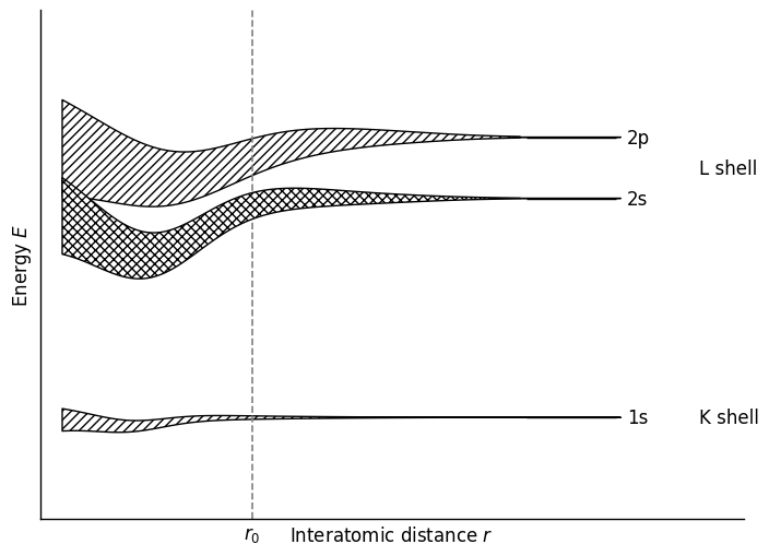
Another concept relevant for understanding chemical bonds is electronegativity which describes the tendency of an atom to attract bonding electrons to itself.

A useful first classification is suggested by chemistry and by periodic-table trends:

• similar electronegativities + strong local orbital overlap \(\rightarrow\) often covalent bonding,
• large electronegativity difference \(\rightarrow\) often ionic bonding,
• spatially extended, partially filled valence states \(\rightarrow\) metallic bonding,
• closed shells or saturated molecules \(\rightarrow\) van der Waals bonding,
• hydrogen bound to strongly electronegative atoms can produce hydrogen bonding.

This classification is only approximate. Real materials often combine several bonding characters. Ionic and covalent bonding, in particular, form a continuum rather than two completely separate categories. Graphite is a classic mixed case: it has strong covalent bonding within the layers and weak van der Waals bonding between them.

Before discussing individual bond types, it is useful to define the cohesive energy. A solid is thermally stable because its total energy is lower than that of the corresponding set of free atoms or molecules. The energy gain due to bonding is

\[ E_{\mathrm{coh}} = E_{\mathrm{free\ atoms}} - E_{\mathrm{solid}} >0. \]

For thermal physics, not only the depth of the energy minimum matters, but also its shape. A deeper and steeper minimum usually implies larger restoring forces, higher vibrational frequencies, and larger characteristic phonon energies.

2.2.1 Covalent Bonding

A covalent bond forms when valence electrons are shared between neighboring atoms instead of being fully transferred from one atom to another. The electron density is concentrated in the region between the two atoms, which makes the bond strongly directional. As a result, bond angles matter just as much as bond lengths. This directionality is why covalent materials such as diamond, silicon, and germanium favor specific local geometries, for example tetrahedral coordination associated with \(sp^3\) hybridization.

A simple microscopic picture comes from the molecular-orbital construction. If \(\Pi_A(\mathbf r)\) and \(\Pi_B(\mathbf r)\) are atomic orbitals centered on atoms \(A\) and \(B\), then the bonding and antibonding combinations are approximated by

\[ \Pi_{\pm}(\mathbf r) = \frac{1}{\sqrt{2 \pm (S_{AB}+S_{AB}^{*})}} \left[ \Pi_A(\mathbf r)\pm \Pi_B(\mathbf r) \right], \]

where \(S_{AB}\) is the overlap integral. The symmetric combination \(\Pi_+\) is the bonding state: it increases electron density between the atoms and lowers the energy. The antisymmetric combination \(\Pi_-\) is the antibonding state.

For a more explicitly two-electron valence-bond picture, the spatial wavefunction of the singlet covalent state is

\[ \Pi_{\mathrm s}(r_1,r_2) = N_+ \left[ \Pi_A(r_1)\Pi_B(r_2)+\Pi_A(r_2)\Pi_B(r_1) \right], \]

with energy

\[ \vartheta_{\mathrm s} = \vartheta_A+\vartheta_B+2N_+^2(C+I), \]

where \(C\) is the direct Coulomb integral and \(I\) the exchange integral. The exchange contribution is essential: it is one of the reasons why the singlet state can develop a minimum at a finite bond length and thus produce binding.

For unlike atoms the bond is often not purely covalent. A useful schematic description is the polar covalent or ionic-covalent bond, where ionic configurations are admixed:

\[ \Pi(r_1,r_2) = N\Big[ \Pi_A(r_1)\Pi_B(r_2)+\Pi_B(r_1)\Pi_A(r_2) +\lambda_A \Pi_A(r_1)\Pi_A(r_2) +\lambda_B \Pi_B(r_1)\Pi_B(r_2) \Big]. \]

This lowers the energy relative to a purely covalent bond and shows why covalent and ionic bonding are not sharply separated.

In a covalent crystal, the total cohesive energy is then built up from a network of such directional bonds. Typical bond energies are a few eV per bond: for example, C–C is about \(3.58\,\mathrm{eV}\), Si–Si about \(2.30\,\mathrm{eV}\), and Ge–Ge about \(1.95\,\mathrm{eV}\).

2.2.2 Ionic Bonding

An ionic bond forms when electrons are transferred from one atom to another because their electronegativities differ strongly. One atom becomes a positively charged cation, the other a negatively charged anion. The dominant attraction is then the long-range Coulomb interaction between these oppositely charged ions. In a crystal this is not just a nearest-neighbor effect: because the Coulomb interaction decays only as \(1/r\), the entire lattice contributes to the binding.

A rough chemical indicator is a large electronegativity difference; in the Pauling scheme, values larger than about \(1.7\) often favor predominantly ionic bonding.

The electrostatic contribution to the energy is the Madelung energy,

\[ E_{\mathrm M} = \frac{1}{2} \sum_{i\neq j} \frac{Z_i Z_j e^2}{4\pi\varepsilon_0 |\mathbf R_i-\mathbf R_j|}. \]

For a binary ionic crystal, this is commonly written per chemical unit as

\[ \frac{E_{\mathrm M}}{N} = -\alpha \frac{Z_1 Z_2 e^2}{4\pi\varepsilon_0 r_0}, \]

where \(r_0\) is the nearest-neighbor cation–anion distance and \(\alpha\) is the Madelung constant, which depends on the lattice geometry.

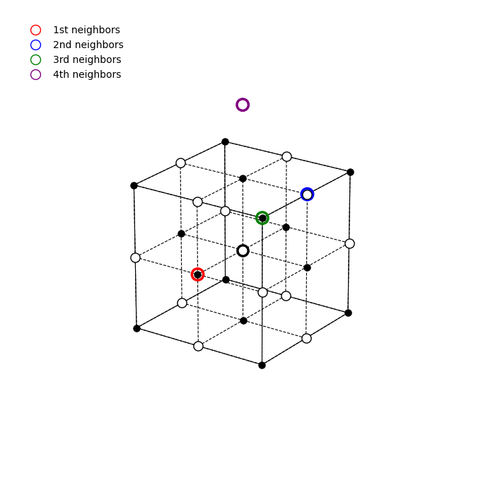
It is determined by summing electrostatic interactions of one reference ion with all other ions in the crystal, taking into account the lattice geometry. For a reference ion at the origin, the Madelung constant is defined as \[ \alpha = \sum_{j\neq 0} \frac{\pm 1}{\frac{r_j}{r_0}}, \] where \(r_j\) is the distance to ion \(j\) measured from the reference ion at the origin, \(r_0\) is the nearest-neighbor distance, and the sign in the numerator is negative for oppositely charged ions and positive for the same charge.

Thus ionic bonding is already an example where structure and bonding are inseparable: NaCl, CsCl, ZnS, and CaF\(_2\) have different Madelung constants because their full ionic environments are different.

Figure 2.2: NaCl crystal structure with first-, second-, third-, and further-neighbor distances, illustrating that the ionic binding energy is a lattice sum rather than a purely local bond.

The Madelung term alone cannot stabilize the crystal. Since it behaves as \(-1/r\), it would predict an unphysical collapse of ions onto one another. At short distances, however, overlapping closed shells produce a strong repulsion, ultimately rooted in the Pauli principle. In ionic solids this is often modeled by the Born–Mayer approximation:

\[ U_{\mathrm{ion}}(r) = -\alpha \frac{Z_1 Z_2 e^2}{4\pi\varepsilon_0 r} + B\exp\!\left(-\frac{r}{\rho}\right). \]

Here \(B\) sets the repulsive energy scale and \(\rho\) its range.

The equilibrium distance \(r_0\) is determined by the minimum condition

\[ \left.\frac{dU_{\mathrm{ion}}}{dr}\right|_{r=r_0} = \alpha \frac{Z_1 Z_2 e^2}{4\pi\varepsilon_0 r_0^2} - \frac{B}{\rho}\exp\!\left(-\frac{r_0}{\rho}\right) = 0. \]

At equilibrium one may eliminate \(B\) and write the energy as

\[ \frac{E}{N} = -\alpha \frac{Z_1 Z_2 e^2}{4\pi\varepsilon_0 r_0} \left( 1-\frac{\rho}{r_0} \right), \]

with \(\rho/r_0\) typically of order \(0.1\).

This is the key thermal message: ionic crystals are stiff because their energy minimum is produced by the balance of a strong long-range attraction and a steep short-range repulsion.

2.2.3 Metallic Bonding

In metals, valence electrons are not tied to individual two-center bonds. Instead, they are spread out over many atoms and form a delocalized electron cloud moving through the crystal of positive ion cores. Metallic bonding is therefore much less directional than covalent bonding, and dense packing becomes especially important.

This delocalization is also the origin of the high electrical and thermal conductivity of metals.

At the present level there is no single simple analytic formula, analogous to the Lennard–Jones or Born–Mayer forms, that captures metallic cohesion in a quantitatively reliable way. One should think instead in terms of a competition between electron kinetic energy, electron-ion attraction, and ion-ion repulsion. Symbolically,

\[ E_{\mathrm{metal}} = E_{\mathrm{electrons}} + E_{\mathrm{electron\mbox{-}ion}} + E_{\mathrm{ion\mbox{-}ion}}. \]

A full treatment requires band theory and the many-electron wavefunction, which is why a detailed calculation of metallic cohesive energies is deferred until the electronic structure of solids is discussed.

For now, the important point is that metallic cohesion is typically intermediate in strength: stronger than van der Waals bonding, but often less directional and less locally concentrated than strong covalent networks.

2.2.4 Van der Waals Bonding

Van der Waals bonding is the weak attraction between closed-shell atoms or saturated molecules. Since there are no unsaturated valence states available for ionic, metallic, or ordinary covalent bonding, the attraction comes from fluctuating and induced dipoles. A temporary dipole on one atom polarizes a neighboring one, and the two attract each other.

At large separations, the interaction energy has the characteristic form

\[ U_{\mathrm{vdW}}(R) = -\frac{C}{R^6}. \]

This \(R^{-6}\) dependence is the hallmark of London dispersion forces.

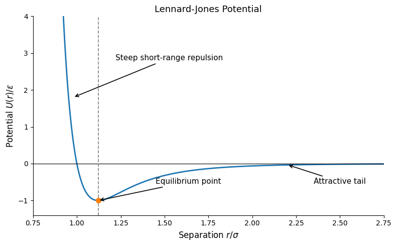
A pure \(-C/R^6\) attraction would again predict collapse at small \(R\), so one adds a short-range repulsive term. A standard empirical model is the Lennard–Jones potential,

\[ U_{\mathrm{LJ}}(r) = 4\varepsilon \left[ \left(\frac{\sigma}{r}\right)^{12} - \left(\frac{\sigma}{r}\right)^6 \right]. \]

Here \(\varepsilon\) sets the depth of the minimum and \(\sigma\) a characteristic length scale.

Figure 2.3: Lennard-Jones potential as a function of separation, showing the attractive tail, the steep short-range repulsion, and the existence of an equilibrium distance at a finite minimum.

For a molecular crystal one sums the pair potentials over the lattice:

\[ E_0 = \frac{1}{2}N\,4\varepsilon \left[ A_{12}\left(\frac{\sigma}{r_0}\right)^{12} - A_6\left(\frac{\sigma}{r_0}\right)^6 \right], \]

where \(r_0\) is the nearest-neighbor distance and the coefficients \(A_6\) and \(A_{12}\) depend on the crystal structure. Minimization yields

\[ r_0 = \left(\frac{2A_{12}}{A_6}\right)^{1/6}\sigma, \qquad \varepsilon_0 = -\frac{A_6^2}{2A_{12}}\varepsilon. \]

Because \(\varepsilon\) is small, van der Waals solids are soft and have low melting temperatures and low characteristic phonon energies.

2.2.5 Hydrogen Bonding

A hydrogen bond forms when hydrogen, already bound to one electronegative atom, also interacts attractively with a second electronegative atom, most commonly O, N, or F. It is therefore a directional secondary bond that combines partial covalent character on one side with weaker attraction on the other. This asymmetry is reflected in the familiar notation

\[ \mathrm{O-H\cdots O}. \]

In ice, for example, the proton is not located exactly at the midpoint between two oxygen atoms, but occupies one of two symmetry-related positions and can oscillate between them.

Unlike the Lennard–Jones or Born–Mayer cases, there is no single simple universal analytic expression used here in these notes for the binding energy of a hydrogen bond. For the present purpose it is enough to characterize hydrogen bonding by its geometry and by its energy scale: it is substantially stronger than a typical van der Waals interaction, but weaker than ordinary covalent or ionic bonding.

In ice, the O–O distance is about \(2.75\,\text{\AA}\) and the energy required to break a hydrogen bond is about \(0.2\,\mathrm{eV}\); for F–H\(\cdots\)F it is about \(0.29\,\mathrm{eV}\).

Hydrogen bonds are central in water, ice, proteins, and DNA, even though they are less central for ordinary inorganic solid-state physics than ionic, covalent, metallic, or van der Waals bonding.

2.2.6 Charge Density: Ionic versus Covalent Bonding

The difference between ionic and covalent bonding can be visualized directly in the electronic charge density.

Figure 2.4: Electron-density contours comparing a typical ionic crystal (NaCl) with a typical covalent crystal (Si). Ionic bonding keeps most charge concentrated around the ions, while covalent bonding builds up charge density along the bond direction.

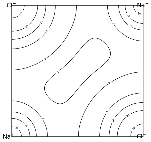
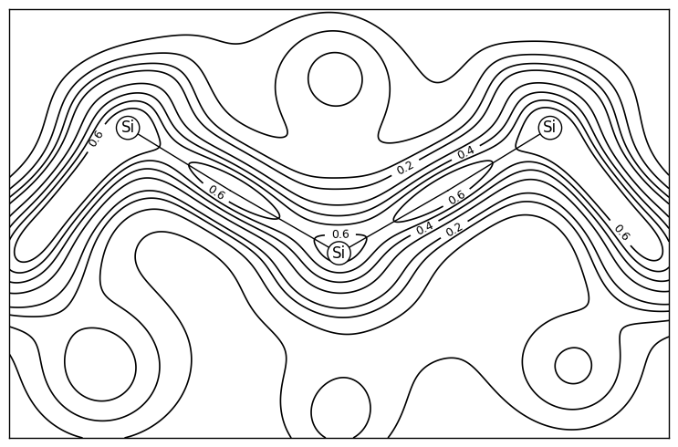
This difference is directly relevant for lattice dynamics: directional charge buildup along bonds usually produces highly anisotropic and comparatively strong restoring forces.

2.2.7 Comparison of Energy Scales

The values quoted below should be read as order-of-magnitude estimates. Depending on context, the literature reports energies per atom, per molecule, or per bond.

Bond Type	Typical Energy Scale	Main Physical Origin	Typical Consequence for Thermal Physics
van der Waals	\(\sim 0.02\)–\(0.2\ \mathrm{eV}\) per atom or molecule	induced dipoles between closed shells / saturated molecules	soft solids, low vibrational frequencies, low melting points
hydrogen	\(\sim 0.1\)–\(0.3\ \mathrm{eV}\) per bond	proton-mediated directional secondary bond	stronger than van der Waals, but still relatively soft
metallic	\(\sim 1\)–\(5\ \mathrm{eV}\) per atom	delocalized valence electrons binding ion cores collectively	moderate to high stiffness; electrons also dominate transport
covalent	typically \(\sim 1.5\)–\(4.5\ \mathrm{eV}\) per bond; often several eV per atom in network solids	charge buildup between neighbors, directional orbital overlap	strong restoring forces, often high phonon frequencies
ionic	typically several eV per chemical unit	long-range Coulomb attraction plus short-range core repulsion	strong cohesion, high stiffness, large characteristic phonon scales

Some representative examples are:

• noble-gas solids: about \(0.1\,\mathrm{eV}\) per atom in order of magnitude,
• hydrogen bonds in ice: about \(0.2\,\mathrm{eV}\) per bond,
• simple metals: typically about \(1\)–\(5\,\mathrm{eV}\) per atom,
• diamond: about \(7.35\,\mathrm{eV}\) per atom,
• silicon: about \(4.66\,\mathrm{eV}\) per atom,
• germanium: about \(3.85\,\mathrm{eV}\) per atom,
• sodium chloride: about \(8.15\,\mathrm{eV}\) per molecule,
• lithium fluoride: about \(10.74\,\mathrm{eV}\) per molecule.

The general trend is clear: weak bonding leads to soft lattices and low thermal energy scales, while strong bonding leads to stiff lattices and high characteristic phonon energies. This is why bonding must be understood before one can understand heat capacity, thermal expansion, and thermal transport in solids.

This form is already enough to see why bonding matters for thermal physics. Once a stable equilibrium distance \(r_0\) exists, the atoms do not remain exactly at rest there. Thermal energy causes small displacements about equilibrium, so the first question is: how does a system behave when it is displaced slightly from a stable minimum?

The prototype for this situation is the harmonic oscillator. Before discussing bond stiffness in a solid, it is therefore useful to recall the basic physics of a mass attached to a spring.

2.3 From the Harmonic Oscillator to Bond Stiffness

2.3.1 Harmonic Oscillator

Consider a particle of mass \(m\) attached to a spring and displaced by an amount \(x\) from its equilibrium position. For small displacements, the restoring force is proportional to the displacement and points back toward equilibrium:

\[ F = -kx . \]

This is Hooke’s law. The constant \(k\) is the spring constant: it measures how strongly the system resists deformation. The minus sign indicates that the force is restoring.

Using Newton’s second law, the equation of motion is

\[ m \ddot x = -kx . \]

Its solution is an oscillatory motion,

\[ x(t) = A \cos(\omega t + \phi), \qquad \omega = \sqrt{\frac{k}{m}} . \]

Thus the oscillation frequency is larger when the restoring force is stronger and smaller when the mass is larger.

The corresponding potential energy is

\[ U(x) = \frac{1}{2} k x^2 . \]

This is a parabola with a minimum at \(x=0\). The harmonic oscillator is therefore the universal model for small oscillations about a stable equilibrium.

2.3.2 Why the Harmonic Oscillator Matters for Solids

A bond in a solid behaves in exactly the same way when the atoms are displaced only slightly from their equilibrium separation. The full interatomic potential \(U(r)\) may have a complicated form, but near its minimum only the local shape matters. In that small region, the potential can be approximated by a parabola, and the atomic motion becomes harmonic to a very good approximation.

This is the key step that connects chemistry to lattice dynamics:
stable bond \(\rightarrow\) restoring force \(\rightarrow\) harmonic vibration.

2.3.3 Equilibrium Distance and Curvature

Let \(U(r)\) be an effective interatomic potential for a given bond. The equilibrium distance \(r_0\) is defined by

\[ \left.\frac{dU}{dr}\right|_{r=r_0}=0 . \]

Near equilibrium, the Taylor expansion is

\[ U(r) = U(r_0) + \frac{1}{2} K_{\mathrm{bond}}(r-r_0)^2 + \mathcal O\left((r-r_0)^3\right), \]

\[ K_{\mathrm{bond}} = \left.\frac{d^2U}{dr^2}\right|_{r=r_0}. \]

The linear term vanishes because \(r_0\) is a minimum. The leading nontrivial term is therefore quadratic, exactly as in the harmonic oscillator.

The quantity

\[ K_{\mathrm{bond}} = \left.\frac{d^2U}{dr^2}\right|_{r=r_0} \]

plays the role of the spring constant. It is the local bond stiffness: it tells us how rapidly the energy rises when the bond is slightly stretched or compressed.

2.3.4 Why Curvature, Not Only Depth, Matters

The depth \(|U(r_0)|\) and the curvature \(K_{\mathrm{bond}}\) are related but not identical.

• A deep minimum means that it costs a lot of energy to separate atoms completely.
• A steep minimum means that even a small displacement away from equilibrium costs a lot of energy.

Thermal vibrations probe the local shape of the minimum, so they depend more directly on \(K_{\mathrm{bond}}\) than on the full dissociation energy alone.

This is why thermal physics must go beyond the simple distinction between “strong” and “weak” bonds. For small vibrations, the relevant quantity is the restoring force near equilibrium, not the total energy required to break the bond completely.

2.3.5 Local Vibrational Frequency Scale

For two atoms with reduced mass \(\mu\), define the relative displacement

\[ x = r-r_0 . \]

In the harmonic approximation,

\[ U(r) \approx U(r_0) + \frac{1}{2}K_{\mathrm{bond}} x^2 . \]

The force is therefore

\[ F = -\frac{dU}{dr} \approx -K_{\mathrm{bond}} x , \]

and the equation of motion for the relative coordinate becomes

\[ \mu \ddot x = -K_{\mathrm{bond}} x , \]

\[ \omega_0 = \sqrt{\frac{K_{\mathrm{bond}}}{\mu}} . \]

This has exactly the same form as the harmonic oscillator, with the replacements

\[ m \rightarrow \mu, \qquad k \rightarrow K_{\mathrm{bond}}. \]

Thus the characteristic vibrational scale increases with

• larger curvature \(K_{\mathrm{bond}}\),
• smaller mass \(\mu\).

This is the central physical message of the lecture.

2.3.6 Interpretation

The formula

\[ \omega_0 = \sqrt{\frac{K_{\mathrm{bond}}}{\mu}} \]

passes two immediate checks:

1. Weak molecular crystal: small \(K_{\mathrm{bond}}\) and often heavy molecules \(\rightarrow\) low-frequency vibrations.
2. Light-element covalent network: large \(K_{\mathrm{bond}}\) and small mass \(\rightarrow\) high-frequency vibrations.

This is why light, strongly covalent solids are natural candidates for large phonon energies, while van der Waals solids are not.

Within the group-IV series, both trends work in the same direction: going from C to Si to Ge, the bond energy decreases while the mass increases, so the vibrational scale should decrease strongly down the group.

2.4 From Local Stiffness to the Debye Scale

A crystal does not vibrate as isolated pairs; it vibrates collectively. Still, the pair picture captures the right scaling. In a lattice, the second derivatives of the total energy with respect to atomic displacements become the force constants. These determine the normal-mode frequencies of the crystal.

For an acoustic branch, the long-wavelength modes are characterized by a sound velocity \(v_s\). Dimensional reasoning gives

\[ v_s \sim a \sqrt{\frac{K_{\mathrm{bond}}}{M}}, \]

where \(a\) is a characteristic spacing and \(M\) is an atomic mass scale. Since the Debye cutoff frequency scales like

\[ \omega_D \sim \frac{v_s}{a}, \]

one obtains the qualitative relation

\[ k_B \Theta_D = \hbar \omega_D, \qquad \Theta_D \propto \sqrt{\frac{K_{\mathrm{bond}}}{M}} . \]

The omitted prefactors depend on structure and dimensionality, but the trend is robust: stiffer bonds and lighter atoms push the Debye temperature upward.

2.4.1 Interpretation

This scaling explains, at a qualitative level, why:

• light covalent solids tend to have high Debye temperatures,
• many ionic and partly covalent ceramics also have comparatively high vibrational scales,
• heavy metals often have lower Debye temperatures than light covalent semiconductors,
• molecular crystals have low Debye temperatures because their intermolecular forces are weak.

It is important not to over-interpret this. A high \(\Theta_D\) signals high characteristic phonon energies, but it does not by itself determine the thermal conductivity. That requires scattering physics, and in metals electronic carriers contribute in addition to phonons.

2.5 Materials Emphasis: Why Ceramics, Metals, and Molecular Crystals Differ Thermally

2.5.1 Ceramics

Many ceramics are dominantly ionic or mixed ionic-covalent solids. Because their bonds are strong, their equilibrium potentials are usually steep near the minimum. As a result, they often have large elastic moduli and comparatively high phonon energy scales.

From a thermal viewpoint, this means:

• high characteristic vibrational frequencies,
• often relatively high Debye temperatures,
• but not automatically high thermal conductivity, because complex structures and disorder can still scatter phonons strongly.

2.5.2 Metals

Metals are bonded by delocalized electrons. Their vibrational stiffness is often moderate rather than extreme, but their thermal behavior is special because electrons carry both charge and heat.

Therefore:

• the lattice part of the thermal scale is not necessarily exceptional,
• yet the total thermal conductivity can be large because of electronic transport,
• and the specific heat acquires both lattice and electronic contributions.

2.5.3 Molecular Crystals

Molecular crystals are held together mainly by van der Waals forces and sometimes supplemented by hydrogen bonds. Their cohesive energies are much smaller than those of ionic or covalent solids.

Hence they are typically:

• soft,
• low-melting,
• rich in low-frequency vibrations,
• low in Debye temperature,
• poor thermal conductors.

2.5.4 A Useful Mixed Case: Graphite

Bonding can differ strongly by direction. In graphite, the bonding is covalent within the layers but only van der Waals between layers.

This immediately implies strong thermal anisotropy:

• stiff, high-frequency motion and efficient heat flow are favored in-plane,
• much softer response is expected perpendicular to the layers.

This example is a good warning against speaking of “the” stiffness of a solid without specifying direction.

Optional / Appendix: Microscopic Models

For ionic solids, the important deeper result is that the Coulomb energy must be summed over the whole crystal, leading to the Madelung constant.

For covalent solids, the Heitler-London and LCAO pictures are often useful for interpretation, where bonding and antibonding states emerge from combining atomic orbitals. The key thermal takeaway is simply that the bonding state concentrates charge between atoms and thereby creates a strong, directional restoring force.

For hybridization, especially \(sp^3\) in diamond-like solids, the main point is structural: bond directionality is built into the electronic wavefunctions themselves.

These microscopic constructions will become useful again later when we discuss why some crystals are especially stiff, anisotropic, or semiconducting.

2.6 Bridge to Lattice Dynamics and the Next Lecture

Today we stayed at the level of bonding curves and characteristic scales. The next lecture replaces the single-coordinate picture \(U(r)\) by the many-atom displacement field of a crystal.

The logical chain is:

1. Choose equilibrium atomic positions.
2. Expand the total crystal energy for small displacements.
3. Keep the quadratic terms: these are the force constants.
4. Solve for the collective normal modes.
5. Interpret the resulting spectrum as phonons.
6. Build from that spectrum the density of states and, later, the heat capacity.

In compact form,

\[ U({ \mathbf u_\ell }) \longrightarrow \frac{\partial^2 U}{\partial u_{\ell \alpha} \partial u_{\ell' \beta}} \longrightarrow \omega_\nu(\mathbf q) \longrightarrow D(\omega) \longrightarrow C_V . \]

The point of today’s lecture is that the entire chain begins with chemistry: bond type sets stiffness, stiffness sets vibrational scales, and vibrational scales set thermal scales.

NoteTake-Home Messages

• The dominant bond type in a solid is strongly constrained by valence-electron structure, electronegativity, and position in the periodic table.
• Covalent, ionic, metallic, van der Waals, and hydrogen bonding differ not only in strength but also in how electronic charge is distributed in space.
• Simple energy models capture the essential physics of several bond types: the Madelung energy for ionic attraction, the Born–Mayer term for short-range ionic repulsion, and the Lennard–Jones potential for van der Waals bonding.
• Cohesive energies span orders of magnitude, from weak molecular-scale binding in van der Waals solids to several eV in ionic and covalent solids.
• Small vibrations about a stable equilibrium are described by the harmonic oscillator, independent of the microscopic origin of the bond.
• The local curvature of the interatomic potential defines the bond stiffness and is more directly relevant for vibrations than the bond energy alone.
• Characteristic vibrational frequencies increase for stiffer bonds and decrease for heavier atoms.
• Debye temperature and many qualitative thermal trends in solids can be traced back to bond type, bond stiffness, and atomic mass, while thermal conductivity also depends on scattering and, in metals, on electronic heat transport.

2.7 Problem Set

1. Bond Types and Microscopic Picture.
   For each of the following solids or bonds, identify the dominant bonding type and briefly describe the corresponding microscopic picture of the electron distribution: solid Ar, ice, NaCl, Cu, Si, and graphite.

2. Ionic Bonding: Madelung Attraction and Born–Mayer Repulsion.
   Consider the model potential for an ionic crystal \[ U_{\mathrm{ion}}(r) = -\alpha \frac{Z_1 Z_2 e^2}{4\pi\varepsilon_0 r} + B\exp\!\left(-\frac{r}{\rho}\right). \]

   1. Explain the physical origin of the two terms.
      
   2. Derive the equilibrium condition that determines the equilibrium distance \(r_0\).
      
   3. Explain why this model already suggests that ionic solids can be relatively stiff.

3. Van der Waals Bonding and the Lennard–Jones Potential.
   The Lennard–Jones potential is \[ U_{\mathrm{LJ}}(r) = 4\varepsilon \left[ \left(\frac{\sigma}{r}\right)^{12} - \left(\frac{\sigma}{r}\right)^6 \right]. \]

   1. Identify which term is attractive and which term is repulsive.
      
   2. Show that the equilibrium distance is \[ r_0 = 2^{1/6}\sigma . \]
   3. Explain why solids held together mainly by van der Waals forces are usually soft and have low characteristic vibrational frequencies.

4. From the Harmonic Oscillator to Bond Stiffness.
   A classical harmonic oscillator obeys \[ m\ddot x = -kx . \]

   1. Write down the corresponding oscillation frequency.
      
   2. For a bond with interatomic potential \(U(r)\) and equilibrium distance \(r_0\), define the bond stiffness \(K_{\mathrm{bond}}\).
      
   3. Show that for two atoms with reduced mass \(\mu\), small oscillations about equilibrium have frequency \[ \omega_0=\sqrt{\frac{K_{\mathrm{bond}}}{\mu}} . \]

5. Energy Scales and Thermal Consequences.
   Put the following bonding types in order of increasing typical energy scale: van der Waals, hydrogen, metallic, covalent, ionic. Then state one thermal consequence of weak bonding and one thermal consequence of strong bonding.

6. Materials Comparison.
   Explain qualitatively why the following classes of materials often differ in their thermal behavior:

   1. ceramics,
      
   2. metals,
      
   3. molecular crystals.
      In your answer, refer to bond type, stiffness, and the carriers responsible for heat transport.